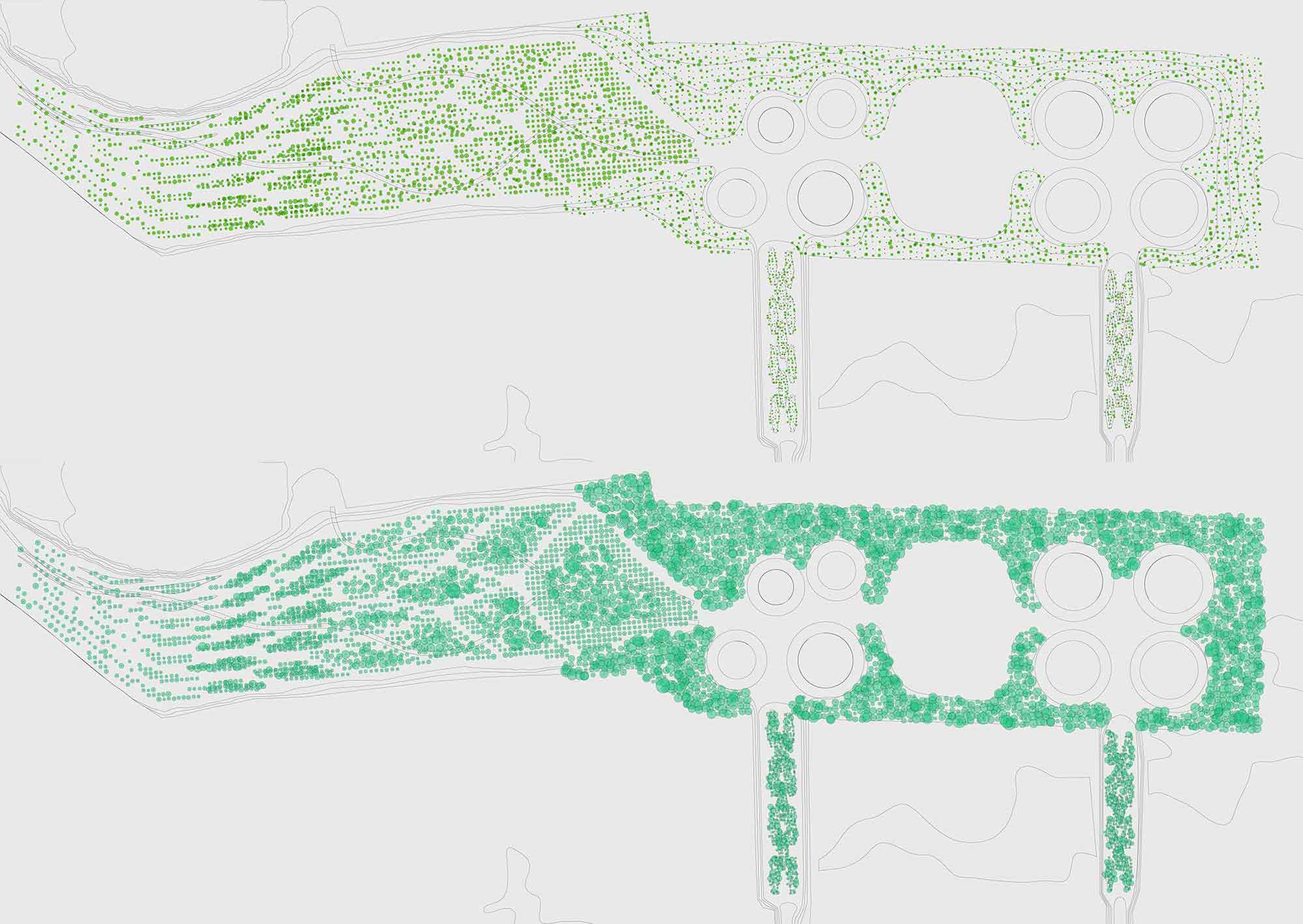
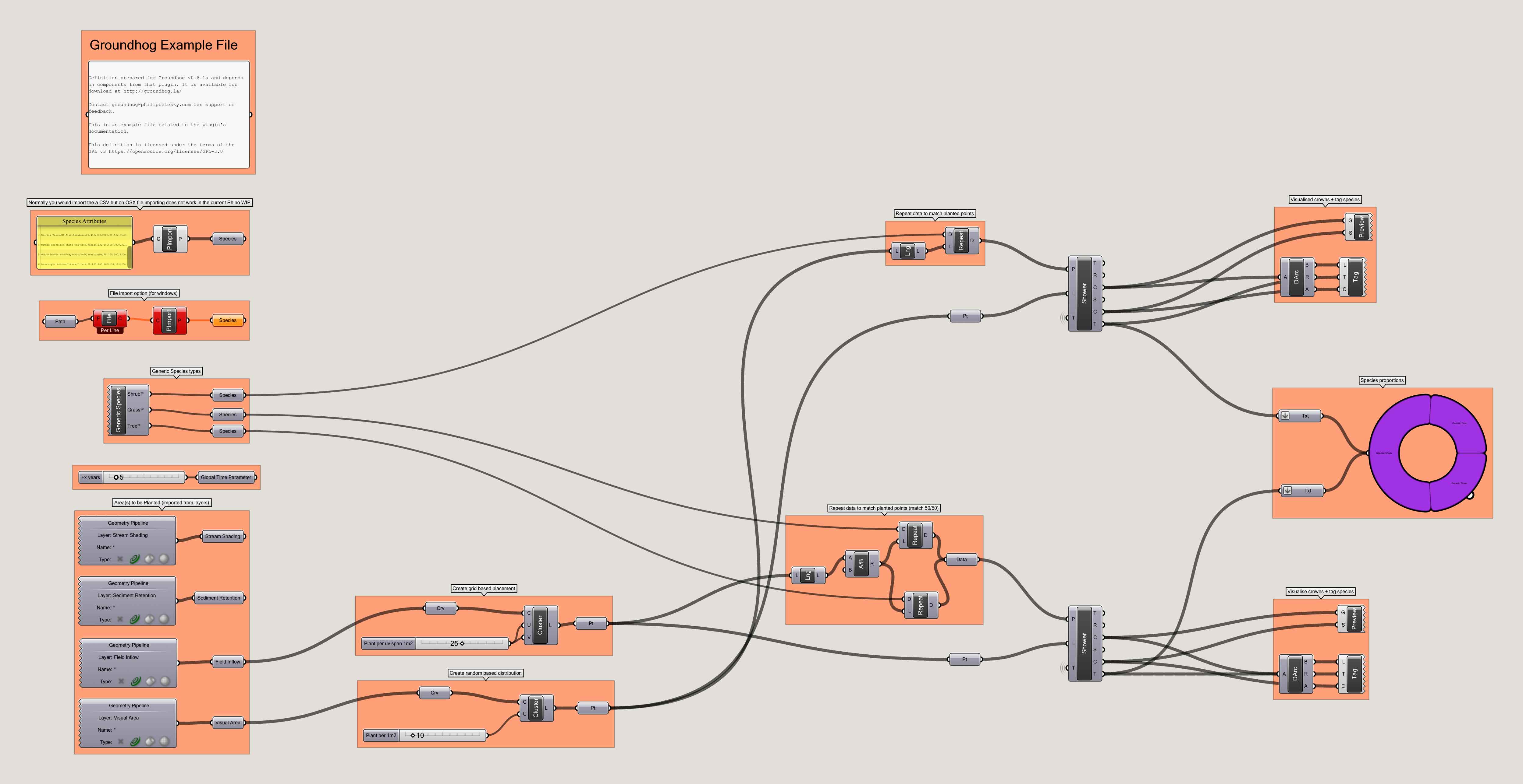
The associated model and definition demonstrating the use of these components can be downloaded here.
Plants
Components that enable the parametric control of plant selection, distribution, performance, and visualisation.
If considered just in terms of its CAD representation, planting design appears to be an exercise in arranging circles. Some circles are smaller or larger, brighter or duller; more round or more frayed. But, after removing the metadata of sprites, colors, and labels, we start and end with a representation of a particular species’ dimensions at maturity: a disc.
It is regrettable that in both digital and analogue mediums the typical representations used poorly reflect their subject matter. Depictions of vegetation are rarely spatially explicit, and often rely on fixed and idealised averages that do not reflect the general nature, or the actual reality, of specific species.12 A plan, once planted, will reach the ‘mature’ state it depicts after years if not decades. This mature state is itself an abstraction, as each plant’s dimensions vary according to the localised conditions that propel or constrain individual growth and are typically altered through ongoing maintenance regimes.

Parametric methods can manage vast quantities of plants distributed across a site and evaluate how they change over time.
Philip Belesky, for https://groundhog.philipbelesky.comWhile many options exist for visualising planting plans with a high degree of fidelity (presuming the correct models for a given species are available) these are typically deployed after the concept design stage, given that they are difficult to implement and modify. As a result, they are often ill-suited to design exploration but useful for evaluating aesthetics.
However, the lack of ‘accurate’ models restricts those earlier stages of the design process, if working in orthographic projections, to the most abstracted versions of a planting plan. This constricts the design potential for vegetated elements in a design, both in terms of their broad visual character, but also in terms of any performance metrics available. Particularly important is the nature of plants as one of the most clearly-evolving elements of a landscape, where growth heavily affects the aesthetics of a space, and so must be planned across different time periods if the space is to be successful before each plant reaches maturity.
Several components in the Groundhog plugin work in conjunction to explore how some aspects of planting design can be eased, or approached differently, using parametric methods. To do so, it augments traditional forms of representations (points and circles) with metadata that describes the spatial and performance characteristics of a particular species. These attributes can then be used to inform the placement of the plants in an automated manner, or be used as analytic tools for better understand how a given plant distribution performs according to specific criteria or over a particular time period.
Plant Palette
Groundhog’s primary input in establishing species attributes is as a spreadsheet; namely namely a CSV file containing tables of information that ready by Grasshopper. The spreadsheet contains a number of ‘core’ and optional parameters for each species that are needed to (later) produce a minimum-viable depiction of the typical geometry and attributes of a species. These values (and example species) are available in the Groundhog - Plants Examples.csv file within the demo files attached to this post. This spreadsheet also provides an easy means of extensibility, where arbitrary values can be added to the definition of each species and then used as part of a parametric model. For example, a value representing phytoremediation potential, or wind breaking potential, could be added to the palette and then used to inform placement or measure performance.
Create plant attributes from an imported spreadsheet
| Mode | Name | ID | Description | Optional | Type |
|---|---|---|---|---|---|
| CSV File |
C
|
The contents of a CSV file (use the output of a Read File component |
GenericParameter
|
||
| Plants |
P
|
The resulting plant objects |
GenericParam
|
A second component contains predefined values for generic forms of vegetation, such as ‘grass’ or ‘shrub’ that enable rapid design prototyping without the need to specify detailed planting characteristics. Similarly, another component is provided for constructing one-off species representations in Grasshopper using explicit parameters, such as for defining canopy radii, rather than needing to always use a spreadsheet-based definition.
Output plant objects from pre-defined generic types
| Mode | Name | ID | Description | Optional | Type |
|---|---|---|---|---|---|
| Shrub |
S
|
Generic Shrub (placeholder data) |
GenericParameter
|
||
| Grass |
G
|
Generic Grass (placeholder data) |
GenericParameter
|
||
| Tree |
T
|
Generic Tree (placeholder data) |
GenericParameter
|
Regardless of which component is used the result is a simple textual representation of the species list, where characteristics use a simple key:value format. This allows the list of species to interact with standard list management tools in Grasshopper for adding/removing/combining species depending on a given logic.
Plant Placement
The next step is related to how plants are distributed across space. This process can proceed using a number of different methods that reflect the varying relationships between landscape conditions and species attributes that drive different planting patterns. At its most simple, the distributor can take a given series of spatial points, developed in Rhinoceros or in Grasshopper as the origin-points for the planting scheme. These can be manually-placed or derived from pre-existing components that define grid patterns, random distributions, etc. More complex options can be assembled by developing further control of point-distributions and how they are matched to the species palette.
Plant Projection
Once a location (in the form of a Point) has been generated for each instance of a species (in the form of the list) these can be fed into the Appearance component. This component then allows for key geometric features of each individual plant to be projected at a specific point in time. At present these visualisation methods are limited to basic circular depictions for criteria such as heights or trunks, root, and canopy radii. While offered as flat linework, many existing Grasshopper tools can be used to assign these projections volume. For instance, the circles that represent canopies can be transformed into spheres or planar surfaces that can then test simple shading effects.
Simulate the appearance of a particular plant instance
| Mode | Name | ID | Description | Optional | Type |
|---|---|---|---|---|---|
| Plants |
P
|
The plant attributes to simulate |
GenericParameter
|
||
| Locations |
L
|
The locations to assign to each attribute |
PointParameter
|
||
| Times |
T
|
The time (in years) since initial planting to display |
NumberParameter
|
||
| Visualisations |
V
|
Whether to show a full L-system visualisation (true) or just the base geoemtries (false) |
BooleanParameter
|
||
| Trunk |
T
|
Trunk radius |
CircleParameter
|
||
| Root |
R
|
Root radius |
CircleParameter
|
||
| Crown |
C
|
Crown radius |
CircleParameter
|
||
| Spacing |
S
|
Spacing radius |
CircleParameter
|
||
| Color |
C
|
The species color of each plant |
ColourParameter
|
||
| Label |
T
|
The species label of each plant |
TextParameter
|
Workflows
While these components are relatively simple in their individual calculations, (especially in the currently-released set of components) their value is as a kit of parts that enables quantitative criteria to be more easily used to design and assess vegetation distributions.
The tripartite attribute/placement/simulation process has emerged from extensive iteration as a means to best support planting design workflows by allowing each task to easily interface with the existing methods available in Grasshopper and its broader plugin ecosystem.

Grasshopper definition demonstrating how to select particular species, place them, and simulate basic growth characteristics.
Philip Belesky, for https://groundhog.philipbelesky.comComing Soon: further components that allow for more naturalistic or performance-based planting distribution and 3D visualisation methods.